Provides correction routines for quasielastic, inelastic and diffraction
reductions.
These interfaces do not support GroupWorkspace’s as input.
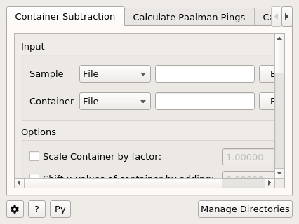
The Container Subtraction Tab is used to remove the container’s contribution to a run.
Once run the corrected output and container correction is shown in the preview plot. Note
that when this plot shows the result of a calculation the X axis is always in wavelength,
however when data is initially selected the X axis unit matches that of the sample workspace.
The input and container workspaces will be converted to wavelength (using
ConvertUnits) if they do not already have wavelength
as their X unit.
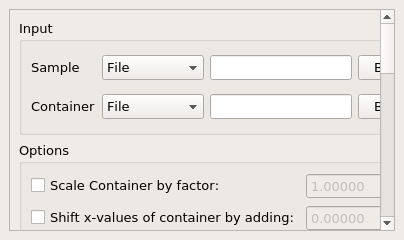
- Sample
- Either a reduced file (_red.nxs) or workspace (_red) or an S(Q,omega) file (_sqw.nxs) or workspace (_sqw) that represents the sample.
- Container
- Either a reduced file (_red.nxs) or workspace (_red) or an S(Q,omega) file (_sqw.nxs) or workspace (_sqw) that represents the container.
- Scale Container by Factor
- Allows the container’s intensity to be scaled by a given scale factor before being used in the corrections calculation.
- Shift X-values by Adding
- Allows the X-values to be shifted by a specified amount.
- Spectrum
- Changes the spectrum displayed in the preview plot.
- Plot Current Preview
- Plots the currently selected preview plot in a separate external window
- Run
- Runs the processing configured on the current tab.
- Plot Spectra
- If enabled, it will plot the selected workspace indices in the selected output workspace.
- Plot Contour
- If enabled, it will plot the selected output workspace as a contour plot.
- Save Result
- If enabled the result will be saved as a NeXus file in the default save directory.
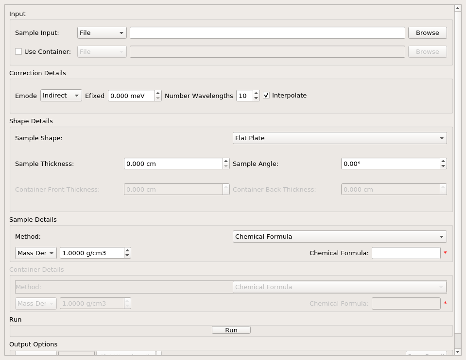
Calculates absorption corrections in the Paalman & Pings absorption factors that
could be applied to the data when given information about the sample (and
optionally the container) geometry.
- Sample Input
- Either a reduced file (_red.nxs) or workspace (_red) or an \(S(Q,
\omega)\) file (_sqw.nxs) or workspace (_sqw).
- Use Container
- If checked allows you to select a workspace for the container in the format of
either a reduced file (_red.nxs) or workspace (_red) or an \(S(Q,
\omega)\) file (_sqw.nxs) or workspace (_sqw).
- Corrections Details
- These options will be automatically preset to the default values read from the sample workspace,
whenever possible. They can be overridden manually.(see below)
- Sample Shape
- Sets the shape of the sample, this affects the options for the shape details
(see below).
- Sample Details Method
- Choose to use a Chemical Formula or Cross Sections to set the neutron information in the sample using
the SetSampleMaterial algorithm.
- Sample/Container Mass density, Atom Number Density or Formula Number Density
- Density of the sample or container. This is used in the SetSampleMaterial
algorithm. If Atom Number Density is used, the NumberDensityUnit property is set to Atoms and if
Formula Number Density is used then NumberDensityUnit is set to Formula Units.
- Sample/Container Chemical Formula
- Chemical formula of the sample or container material. This must be provided in the
format expected by the SetSampleMaterial
algorithm.
- Cross Sections
- Selecting the Cross Sections option in the Sample Details combobox will allow you to enter coherent,
incoherent and attenuation cross sections for the Sample and Container (units in barns).
- Run
- Runs the processing configured on the current tab.
- Plot Wavelength
- If enabled, it will plot a wavelength spectrum represented by the selected workspace indices.
- Plot Angle
- If enabled, it will plot an angle bin represented by the neighbouring bin indices.
- Save Result
- Saves the result in the default save directory.
- Emode
- The energy transfer mode. All the options except Efixed require the input workspaces to be in wavelength.
In Efixed mode, correction will be computed only for a single wavelength point defined by ` Efixed` value.
All the options except Elastic require the Efixed value to be set correctly.
For flat plate, all the options except Efixed, are equivalent.
In brief, use Indirect for QENS, Efixed for FWS and diffraction.
Efixed can be used for QENS also, if the energy transfer can be neglected compared to the incident energy.
See CylinderPaalmanPingsCorrections for the details.
- Efixed
- The value of the incident (indirect) or final (direct) energy in mev. Specified in the instrument parameter file.
- Number Wavelengths
- Number of wavelength points to compute the corrections for. Ignored for Efixed.
- Interpolate
- Whether or not to interpolate the corrections as a function of wavelength. Ignored for Efixed.
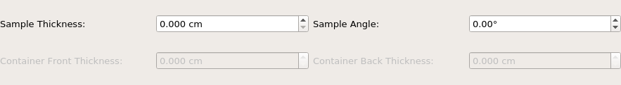
Depending on the shape of the sample different parameters for the sample
dimension are required and are detailed below.
The calculation for a flat plate geometry is performed by the
FlatPlatePaalmanPingsCorrection
algorithm.
- Sample Thickness
- Thickness of sample in \(cm\).
- Sample Angle
- Angle of the sample to the beam in degrees.
- Container Front Thickness
- Thickness of front container in \(cm\).
- Container Back Thickness
- Thickness of back container in \(cm\).
The calculation for a cylindrical geometry is performed by the
CylinderPaalmanPingsCorrection
algorithm.
- Sample Inner Radius
- Radius of the inner wall of the sample in \(cm\).
- Sample Outer Radius
- Radius of the outer wall of the sample in \(cm\).
- Container Outer Radius
- Radius of outer wall of the container in \(cm\).
- Beam Height
- Height of incident beam \(cm\).
- Beam Width
- Width of incident beam in \(cm\).
- Step Size
- Step size used in calculation in \(cm\).
The main correction to be applied to neutron scattering data is that for
absorption both in the sample and its container, when present. For flat plate
geometry, the corrections can be analytical and have been discussed for example
by Carlile [1]. The situation for cylindrical geometry is more complex and
requires numerical integration. These techniques are well known and used in
liquid and amorphous diffraction, and are described in the ATLAS manual [2].
The absorption corrections use the formulism of Paalman and Pings [3] and
involve the attenuation factors \(A_{i,j}\) where \(i\) refers to
scattering and \(j\) attenuation. For example, \(A_{s,sc}\) is the
attenuation factor for scattering in the sample and attenuation in the sample
plus container. If the scattering cross sections for sample and container are
\(\Sigma_{s}\) and \(\Sigma_{c}\) respectively, then the measured
scattering from the empty container is \(I_{c} = \Sigma_{c}A_{c,c}\) and
that from the sample plus container is \(I_{sc} = \Sigma_{s}A_{s,sc} +
\Sigma_{c}A_{c,sc}\), thus \(\Sigma_{s} = (I_{sc} - I_{c}A_{c,sc}/A_{c,c}) /
A_{s,sc}\).
References:
- C J Carlile, Rutherford Laboratory report, RL-74-103 (1974)
- A K Soper, W S Howells & A C Hannon, RAL Report RAL-89-046 (1989)
- H H Paalman & C J Pings, J Appl Phys 33 2635 (1962)
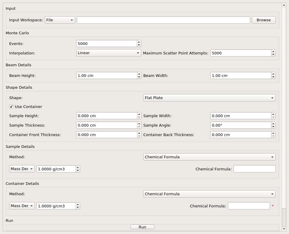
The Calculate Monte Carlo Absorption tab provides a cross platform alternative to the
Calculate Paalman Pings tab. In this tab a Monte Carlo implementation is used to calculate the
absorption corrections.
- Workspace Input
- Either a reduced file (_red.nxs) or workspace (_red) or an \(S(Q,
\omega)\) file (_sqw.nxs) or workspace (_sqw).
- Number Wavelengths
- The number of wavelength points for which a simulation is attempted.
- Events
- The number of neutron events to generate per simulated point.
- Interpolation
- Method of interpolation used to compute unsimulated values.
- Maximum Scatter Point Attempts
- Maximum number of tries made to generate a scattering point within the sample (+ optional
container etc). Objects with holes in them, e.g. a thin annulus can cause problems if this
number is too low. If a scattering point cannot be generated by increasing this value then
there is most likely a problem with the sample geometry.
- Beam Height
- The height of the beam in \(cm\).
- Beam Width
- The width of the beam in \(cm\).
- Shape Details
- Select the shape of the sample (see specific geometry options below). Alternatively, select ‘Preset’ to use the Sample and Container geometries defined on the input workspace.
- Use Container
- If checked, allows you to input container geometries for use in the absorption corrections.
- Sample Details Method
- Choose to use a Chemical Formula or Cross Sections to set the neutron information in the sample using
the SetSampleMaterial algorithm.
- Sample/Container Mass density, Atom Number Density or Formula Number Density
- Density of the sample or container. This is used in the SetSampleMaterial
algorithm. If Atom Number Density is used, the NumberDensityUnit property is set to Atoms and if
Formula Number Density is used then NumberDensityUnit is set to Formula Units.
- Sample/Container Chemical Formula
- Chemical formula of the sample or container material. This must be provided in the
format expected by the SetSampleMaterial
algorithm.
- Cross Sections
- Selecting the Cross Sections option in the Sample Details combobox will allow you to enter coherent,
incoherent and attenuation cross sections for the Sample and Container (units in barns).
- Run
- Runs the processing configured on the current tab.
- Plot Wavelength
- If enabled, it will plot a wavelength spectrum represented by the selected workspace indices.
- Plot Angle
- If enabled, it will plot an angle bin represented by the neighbouring bin indices.
- Save Result
- Saves the result in the default save directory.
Depending on the shape of the sample different parameters for the sample
dimension are required and are detailed below.
This option will use the Sample and Container geometries as defined in the input workspace. No further geometry inputs will be taken, though the Sample material can still be overridden.
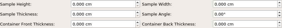
Flat plate calculations are provided by the
IndirectFlatPlateAbsorption algorithm.
- Sample Width
- Width of the sample in \(cm\).
- Sample Height
- Height of the sample in \(cm\).
- Sample Thickness
- Thickness of the sample in \(cm\).
- Sample Angle
- Angle of the sample to the beam in degrees.
- Container Front Thickness
- Thickness of the front of the container in \(cm\).
- Container Back Thickness
- Thickness of the back of the container in \(cm\).
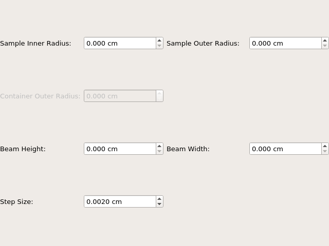
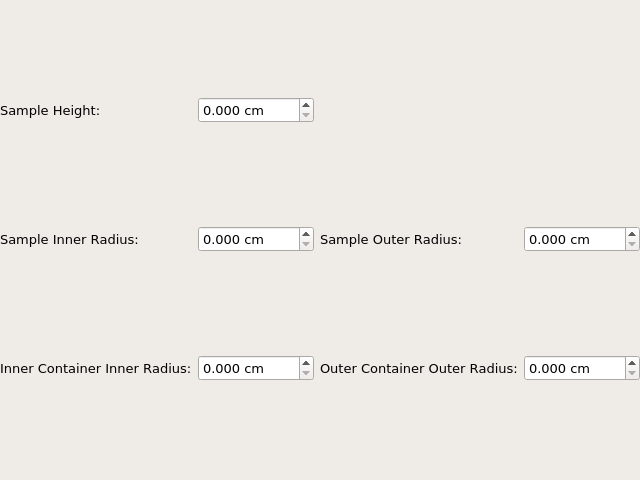
Annulus calculations are provided by the IndirectAnnulusAbsorption algorithm.
- Sample Inner Radius
- Radius of the inner wall of the sample in \(cm\).
- Sample Outer Radius
- Radius of the outer wall of the sample in \(cm\).
- Container Inner Radius
- Radius of the inner wall of the container in \(cm\).
- Container Outer Radius
- Radius of the outer wall of the container in \(cm\).
- Sample Height
- Height of the sample in \(cm\).
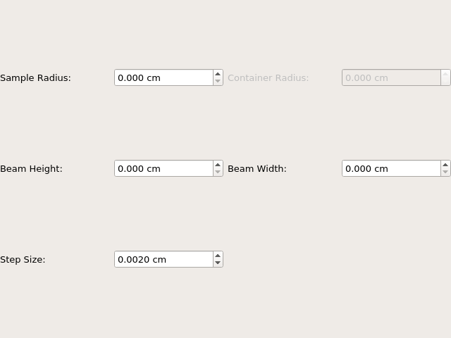
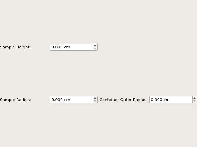
Cylinder calculations are provided by the
IndirectCylinderAbsorption algorithm.
- Sample Radius
- Radius of the outer wall of the sample in \(cm\).
- Container Radius
- Radius of the outer wall of the container in \(cm\).
- Sample Height
- Height of the sample in \(cm\).
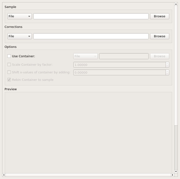
The Apply Corrections tab applies the corrections calculated in the Calculate Paalman
Pings or Calculate Monte Carlo Absorption tabs of the Indirect Data Corrections interface.
This uses the ApplyPaalmanPingsCorrection algorithm to apply absorption corrections in
the form of the Paalman & Pings correction factors. When Use Container is disabled
only the \(A_{s,s}\) factor must be provided, when using a container the
additional factors must be provided: \(A_{c,sc}\), \(A_{s,sc}\) and
\(A_{c,c}\).
Once run the corrected output and container correction is shown in the preview plot. Note
that when this plot shows the result of a calculation the X axis is always in
wavelength, however when data is initially selected the X axis unit matches that
of the sample workspace.
The input and container workspaces will be converted to wavelength (using
ConvertUnits) if they do not already have wavelength
as their X unit.
The binning of the sample, container and corrections factor workspace must all
match, if the sample and container do not match you will be given the option to
rebin (using RebinToWorkspace) the sample to
match the container, if the correction factors do not match you will be given
the option to interpolate (SplineInterpolation) the correction factor to match the sample.
- Sample
- Either a reduced file (_red.nxs) or workspace (_red) or an \(S(Q,
\omega)\) file (_sqw.nxs) or workspace (_sqw).
- Corrections
- The calculated corrections workspace produced from one of the preview two tabs.
- Geometry
- Sets the sample geometry (this must match the sample shape used when calculating
the corrections).
- Use Container
- If checked allows you to select a workspace for the container in the format of
either a reduced file (_red.nxs) or workspace (_red) or an \(S(Q,
\omega)\) file (_sqw.nxs) or workspace (_sqw).
- Scale Container by factor
- Allows the container intensity to be scaled by a given scale factor before
being used in the corrections calculation.
- Shift X-values by Adding
- Allows the X-values of the container to be shifted by a specified amount.
- Rebin Container to Sample
- Rebins the container to the sample.
- Spectrum
- Changes the spectrum displayed in the preview plot.
- Plot Current Preview
- Plots the currently selected preview plot in a separate external window
- Run
- Runs the processing configured on the current tab.
- Plot Spectra
- If enabled, it will plot the selected workspace indices in the selected output workspace.
- Plot Contour
- If enabled, it will plot the selected output workspace as a contour plot.
- Save Result
- If enabled the result will be saved as a NeXus file in the default save directory.
Categories: Interfaces | Indirect